Survival Analysis

Survival data characteristics

in survival data, the labels are amounts of time to event
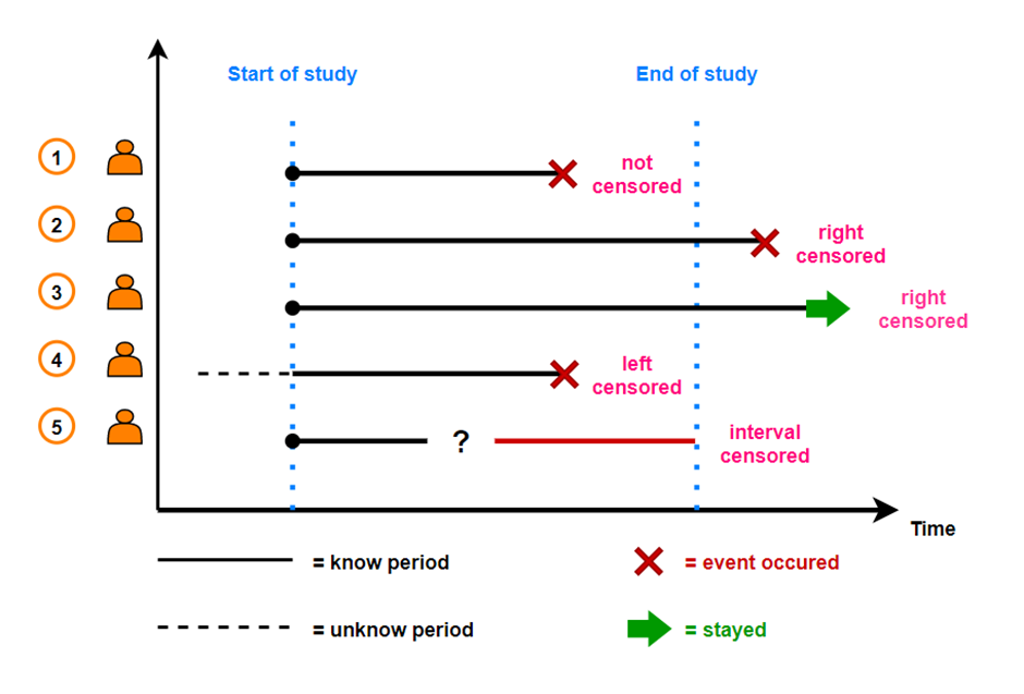
censoring observations: no observations of events happening in the specified time period:
- end-of-study censoring (no event)
- loss-to-follow-up censoring (patients withdraw)
- left censoring = the time to events is only known to before a certain value
- right censoring = the time to events is only known to exceed a certain value (e.g. 12 months → 12m +)
  
  (image source)

Survival function

= the probability of survival past any time t:

S (t) = P r (T > t)

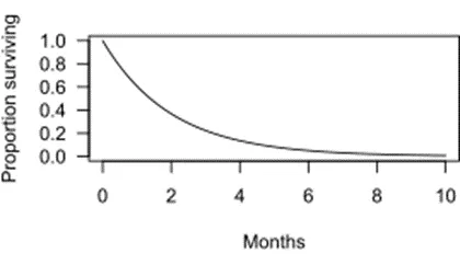
always decreasing from 1 to 0: longer the t, harder to survive:

(image source)
There are parametric and non-parametric models for the survival function. Non-parametric models are mostly used in survival analysis (ref).

Parametric Survival models

The Uniform Model (De-Moivre’s)
Exponential Model
The Gompertz model
The Modified Gompertz Model (Makeham Model)
The Weibull Model

Non-Parametric Models

Kaplan Meier Model

= the probability of survival past t months with censored observations:

S (t) = \prod 1 - P r (T = i | T >= i) = \prod_{t_{i} \leq t} (1 - \frac{d_{i}}{n_{i}})

where

$t_{i}$ are the events observed in the dataset
$d_{i}$ is the number of deaths at time $t_{i}$
$n_{i}$ is the number of people who we know have survived up to time $t_{i}$ .

Important

Note that Kaplan-Meier estimator estimates the survival function directly from observed data, making no assumptions about the underlying hazard function.

Hazard Function

= the instantaneous rate of death at time $t$ , given that the subject has survived up to that time
= the chances of dying in a small interval of time:

h (t) = l i m_{Δ t \to 0} \frac{P (t \leq T < t + Δ t | T \geq t)}{Δ t}

cumulative hazard

H (t) = \int _0 {#t} h(t) dt

relation between survival and hazard

S(t) = exp(- \int _0 {#t} h(t) dt)

Cox (Proportional Hazards) Model

= a regression model for survival data that allows us to assess the effect of covariates on survival time while making minimal assumptions about the shape of the hazard function:

h (t | X) = h_{0} (t) e x p (β_{1} X_{1} + β_{2} X_{2} + . . . + β_{p} X_{p})

where

$h (t | X)$ is the hazard function for a subject with covariate values $X$
$h_{0} (t)$ is the baseline hazard function (the hazard function when all covariates are zero)
$β_{1}, β_{2}, . . ., β_{p}$ are the regression coefficients associated with covariates $X_{1}, X_{2}, . . . X_{p}$ , respectively.

Inspiring

In other words, it is similar to Multiple Regression Analysis, but the difference is that the depended variable is the Hazard Function at a given time t.

When facing many features, we should consider Penalized Cox Models, and the penalization/regularization techniques are similar to linear regression:

Tree-structured Survival Models

Tree-structured

assumptions
- Cox model assumes proportional hazards, meaning the effect of covariates is constant over time.
- survival trees does not rely on the proportional hazards assumption
non-linear relationship and high-dimensional data
- Cox model cannot handle non-linear relationship and can struggle with high-dimensional data
- survival trees can handle both

Survival trees

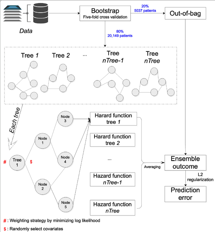
The single survival tree prediction for an individual is a cumulative hazard function (CHF) computed for all individuals in the same tree terminal node:

H_{h} (t) = \sum_{t_{l}, h \leq t} \frac{d_{l}, h}{R_{l}, h}

where $h$ is terminal node, $t$ is event time, $d$ is the number of events at time $t$ , and $R$ is the number of individuals at risk at time $t$ .

Survival random forest

With the CHF for each tree defined above, the entire forest the CHF averaged over all trees:

H(t|x) = \frac{1}{N} \sum _{i=1} {#N} H_i(t|x)

where $H_{i}$ is the estimated CHF for the individual x's terminal node in the $i$ -th of the N trees.

image source

Deep Learning Survival Models

#TODO

Example of usage

Given such a dataset:

Subject	Time (months)	Event	Age (years)	Gender	Treatment
1	10	1	55	M	Drug A
2	15	1	62	F	Drug B
3	20	0	48	M	Drug A
4	25	1	70	F	Drug A
5	30	0	58	M	Drug B

To describe the survival time:
- Kaplan-Meier Estimator can be used to estimate the survival function for each treatment group
- Hazard function can be used to estimate the hazard rate changes over time for each treatment group
To describe the effect of variables on survival:
- Cox proportional hazards model can be used to assess the effect of treatment on survival, while controlling for age and gender

Model evaluation

Graphical Evaluation

Kaplan-Meier Curves
Cox-Snell Residual Plot

Measure the discrimination ability of survival models

Concordance Index (C-index, or Harrell's C-index)

= quantifies the model's ability to correctly rank the relative risks or predicted survival probabilities of pairs of subjects:

\frac{# c o n c o r d a n t p a i r s + 0.5 \times # r i s k t i e s}{# p e r m i s s i b l e p a i r s}

How is it computed:
1. For each pair of subjects in the dataset, compare their predicted survival times or risk scores
2. count concordant pair: the subject with the higher predicted survival time or lower risk score also experiences the event (e.g., death) first
3. count discordant pair: If the subject with the higher predicted survival time or lower risk score does not experience the event first
4. count tied pair: the predicted survival times or risk scores are equal for a pair of subjects
5. C-index is then calculated as the proportion of concordant pairs among all non-tied pairs:
The C-index ranges from 0.5 to 1.0:
- 0.5 = random choice
- 1.0 = perfect discrimination

Time-dependent Area Under the Curve (AUC)

= the AUC for different time points to assess the model's predictive accuracy over time